14. FUNCTION Namelist

14.1. Overview

There is often a need to specify phase properties, boundary condition data, source data, etc., as functions rather than constants. The FUNCTION namelist provides a means for defining functions that can be used in many situations.

The namelist can define several types of functions: a multi-variable polynomial, a continuous piecewise linear function defined by a table of values, a smooth step function, and with certain Truchas build configurations, a general user-provided function from a shared object library that is dynamically loaded at runtime. The functions are functions of \(m\) variables. The expected number of variables and what unknowns they represent (i.e., temperature, time, x-coordinate, etc.) depends on the context in which the function is used, and this will be detailed by the documentation of those namelists where these functions can be used.

Polynomial Function This function is a polynomial in the variables \(v = (v_1,.....,v_m)\) of the form

(14.1.1)\[f(v) = \sum_{j=1}^{n} c_j \prod_{i=1}^{m}(v_i - a_i)^{(e_{ij})}\]

with coefficients \(c_j\), integer-valued exponents \(e^{ij}\), and arbitrary reference point \(a= (a_1,...,a_m)\). The coefficients are specified by Poly_Coefficients, the exponents by Poly_Exponents, and the reference point by Poly_Refvars.

Tabular Function This is a continuous, single-variable function \(y = f(x)\) interpolated from a sequence of data points \((x_i,y_i), i= 1,...,n,\) with \(x_i < x_i+1\). A smooth interpolation method is available in addition to the standard linear interpolation; see Tabular_Interp. There are also two different methods for extrapolating on \(x < x_1\) and \(x > x_n\); see Tabular_Extrap.

Smooth Step Function This function is a smoothed \((C_1)\) step function in a single variable \(v= (x)\) of the form

\[ f(x) = \left\{ \begin{array}{ @{}% no padding l@{\quad}% some padding r@{}% no padding >{{}}r@{}% no padding >{{}}l@{}% no padding } y_0,& if &x \leq x_0 \\ y_0 + (y_1 - y_0) s^2 (3-2s), s \equiv (x - x_0)/(x_1 - x_0), & when &x \in (x_0, x_1) \\ y_1,& if &x \geq x_1, \end{array} \right. \]

with parameters \(x_0\), \(x_1\), \(y_0\), and \(y_1\)

Shared Library Function This is a function from a shared object library having a simple Fortran 77 or C compatible interface. Written in Fortran 77 the function interface must look like

double precision function myfun (v, p) bind(c)

double precision v(*), p(*)

where myfunc can, of course, be any name. The equivalent C interface is

double myfun (double v[], double p[]);

The vector of variables \(v= (v_1,...,v_m)\) is passed in the argument \(v\) and a vector of parameter values specified by Parameters is passed in the argument \(p\). Instructions for compiling the code and creating a shared object library can be found in the Truchas Installation Guide. The path to the library is given by Library_Path and the name of the function (myfun, e.g.) is given by Library_Symbol. Note that the bind(c) attribute on the function declaration inhibits the Fortran compiler from mangling the function name (by appending an underscore, for example) as it normally would.

14.2. FUNCTION Namelist Features

Required/Optional : Optional
Single/Multiple Instances: Multiple

14.3. Components

Name

Description : A unique name by which this function can be referenced by other namelists.
Type : A case-sensitive string of up to 31 characters.
Default : None

Type

Description : The type of function defined by the namelist.
Type : A case-sensitive string
Default : None
Valid Values: “polynomial” for a polynomial function,”tabular” for a tabular function,”smooth step” for a smooth step function, or “library” for a function from a shared object library. The “library” value is not available with a Truchas executable built with the “dynamic loading” option disabled.

Library_Path

Description : The path to the shared object library that contains the function.
Type : A string of up to 128 characters.
Default : None

Library_Symbol

Description : The symbol name of the function within the shared object file.
Type : A string of up to 128 characters.
Default : None
Notes : Unless the Fortran function is declared with the BIND(C) attribute, which is the recommended practice, a Fortran compiler will almost always mangle the name of the function so that the symbol name is not quite the same as the name in the source code. Use the UNIX/Linux command-line utility nm to list the symbol names in the library file to determine the correct name to use here.

Parameters

Description : Optional parameter values to pass to the shared library function.
Type : real vector of up to 16 values
Default : None

Poly_Coefficients

Description : The coefficients \(c_j\) of the polynomial Eq.14.1.1
Type : real vector of up to 64 values
Default : None

Poly_Exponents

Description : The exponents \(e_{ij}\) of the polynomial Eq.14.1.1
Type : integer array
Default : None
Notes : Namelist array input is very flexible. The syntax

Poly_Exponents(i,j) = .....

defines the value for exponent \(e_{ij}\). All the variable exponents for coefficient \(j\) can be defined at once by listing their values with the syntax

Poly_Exponents(:,j) = .....

In some circumstances it is possible to omit providing 0-exponents for variables that are unused. For example, if the function is expected to be a function of (t,x,y,z), but a polynomial in only t is desired, one can just define a 1-variable polynomial and entirely ignore the remaining variables. On the other hand, if a polynomial in z is desired, one must specify 0-valued exponents for all the preceding variables.

Poly_Refvars

Description : The optional reference point a of the polynomial Eq.14.1.1
Type : real vector
Default : 0.0

Tabular_Data

Description : The table of values \((x_i,y_i)\) defining a tabular function \(y=f(x)\). See also Tabular_Dim, Tabular_Interp, and Tabular_Extrap for additional variables that define the function.
Type : real array
Default : None
Notes : This is a \(2 × n\) array with \(n \leq 100\). Namelist array input is very flexible and the values can be specified in several ways. For example, the syntax
Tabular_Data(1,:) = x_1, x_2, ......., x_n
Tabular_Data(2,:) = y_1, y_2, ......., y_n

specifies the \(x_i\) and \(y_i\) values as separate lists. Or the values can be input naturally as a table

Tabular_Data = x_1, y_1
               x_2, y_2
               ...
               x_n, y_n

The line breaks are unnecessary, of course, and are there only for readability as a table.

Tabular_Dim

Description : The dimension in the m-vector of independent variables that serves as the independent variable for the single-variable tabular function.
Type : integer
Default : 1
Notes : Functions defined by this namelist are generally functions of m variables \((v_1,v_2,...,v_m)\). The number of variables and the unknowns to which they correspond depend on the context where the function is used. One of these variables needs to be selected to be the independent variable used for the tabular function. In typical use cases the desired tabular function will depend on time or temperature. Those unknowns are often the first variable, and the default value of Tabular_Dim is appropriate.

Tabular_Extrap

Description : Specifies the method used for extrapolating outside the range of tabular function data points.
Type : case-insensitive string
Default : “nearest”
Valid values: “nearest”, “linear”
Notes : Nearest extrapolation continues the \(y\) value at the first or last data point. Linear extrapolation uses the slope of the first or last data interval, or if Akima smoothing is used (see Tabular_Interp) the computed slope at the first or last data point.

Tabular_Interp

Description : Specifies the method used for interpolating between tabular function data points.
Type : case-insensitive string
Default : “linear”
Valid values: “linear”, “akima”
Notes : Akima interpolation [1] uses Hermit cubic interpolation on each data interval, with the slope at each data point computed from the linear slopes on the neighboring four intervals. The resulting function is \(C^1\) smooth. To determine the slope at the first two and last two data points, two virtual data intervals are generated at the beginning and at the end using quadratic extrapolation. The algorithm seeks to avoid undulations in the interpolated function where the data suggests a flat region though its choice of slopes at data points. Figure 14.3.1 A shows the typical smooth Akima interpolation. If the first interval was expected to be flat, the exhibited undulation would likely be unacceptable. By inserting an additional data point to create successive intervals with the same slope, as in Figure 14.3.1 BC, the algorithm identifies it as a flat region and preserves it in the interpolation. Where two flat regions with differing slopes meet, it is impossible to simultaneously retain smoothness and preserve flatness. In this case a modification to the Akima algorithm used by Matlab’s tablelookup function is adopted, which gives preference to the region with smaller slope as shown in Figure 14.3.1 D
../_images/akima.png

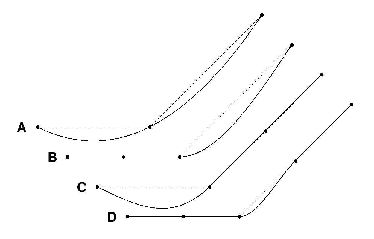
Figure 14.3.1 Examples of smooth Akima interpolation.

Smooth_Step_X0

Description : The parameter \(x_0\) of the function Eq.14.1.2
Type : real
Default : none
Valid values: Require only \(x_0 \leq x_1\).

Smooth_Step_X1

Description : The parameter \(x_1\) of the function Eq.14.1.2
Type : real
Default : none
Valid values: Require only \(x_0 \leq x_1\).

Smooth_Step_Y0

Description : The parameter \(y_0\) of the function Eq.14.1.2
Type : real
Default : none

Smooth_Step_Y1

Description : The parameter \(y_1\) of the function Eq.14.1.2
Type : real
Default : none